hatch 生成边界 |
您所在的位置:网站首页 › hatch hatch › hatch 生成边界 |
hatch 生成边界
定义和符号 (Definitions and Notations)
B(bounding box) :- [x1,y1,x2,y2]LT(top left)-[x1,y1] and BR(bottom right)-[x2,y2]B’:- Generated bounding boxB:- Ground truth bounding box
 link]
链接 ]
link]
链接 ]
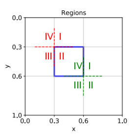
Fig-3 Depicts different regions. Boundary points are generated for each region separately. 图3描述了不同的区域。 分别为每个区域生成边界点。 1.1 findTopLeftPointBorders (1.1 findTopLeftPointBorders)The top left boundary points are generated separately in four regions(refer to Fig-3). Each region produces an array of points(x1’,y1’) given ground truth bounding box and T(IoU threshold). 左上边界点在四个区域中分别生成(请参阅图3)。 给定地面真值边界框和T(IoU阈值),每个区域都会生成一个点数组(x1',y1')。 Fig-4 [a,b,c,d] provides region-wise equations for boundary point generation based on which code is written and output is generated. 图4 [a,b,c,d]提供了边界点生成的区域方程式,基于该方程式编写了代码并生成了输出。 Atributes Required:box, ##Ground Truth boxIoU, ##T- IoU threshouldboxArea ## area of gound truth box source) of Quadrant 1
源 )
#1st Quadrant BoundingPoints Generation x1TR = np.arange(box[0], box[2] - IoU * (box[2] - box[0]), step=IoULimitPrecision)I = (box[2] - x1TR) * (box[3] - box[1])y1TR = box[3] - (I / IoU - boxArea + I) / (box[2] - x1TR)
source) of Quadrant 1
源 )
#1st Quadrant BoundingPoints Generation x1TR = np.arange(box[0], box[2] - IoU * (box[2] - box[0]), step=IoULimitPrecision)I = (box[2] - x1TR) * (box[3] - box[1])y1TR = box[3] - (I / IoU - boxArea + I) / (box[2] - x1TR)
 source) of Quadrant 2
信号源 )
#2nd Quadrant Boundary Points Generationy1BR = np.arange(box[1], box[3] - (boxArea * IoU) / (box[2] - box[0]), step=IoULimitPrecision)x1BR = box[2] - ((boxArea * IoU) / ((box[3] - y1BR)))
source) of Quadrant 2
信号源 )
#2nd Quadrant Boundary Points Generationy1BR = np.arange(box[1], box[3] - (boxArea * IoU) / (box[2] - box[0]), step=IoULimitPrecision)x1BR = box[2] - ((boxArea * IoU) / ((box[3] - y1BR)))
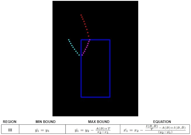 source) of Quadrant 3
信号源 )
#3rd Quadrant Boundary Points Generationy1BL = np.arange(box[1], box[3] - (boxArea * IoU) / (box[2] - box[0]), step=IoULimitPrecision)I = (box[2] - box[0]) * (box[3] - y1BL)x1BL = box[2] - (I / IoU - boxArea + I) / (box[3] - y1BL)inv_idx = np.arange(y1BL.shape[0] - 1, -1, -1).astype(int)y1BL = y1BL[inv_idx]x1BL = x1BL[inv_idx]
source) of Quadrant 3
信号源 )
#3rd Quadrant Boundary Points Generationy1BL = np.arange(box[1], box[3] - (boxArea * IoU) / (box[2] - box[0]), step=IoULimitPrecision)I = (box[2] - box[0]) * (box[3] - y1BL)x1BL = box[2] - (I / IoU - boxArea + I) / (box[3] - y1BL)inv_idx = np.arange(y1BL.shape[0] - 1, -1, -1).astype(int)y1BL = y1BL[inv_idx]x1BL = x1BL[inv_idx]
 source) of Quadrant 4
信号源 )
#4th Quadrant Boundary Points Generationy1TL = np.arange((((box[3] * (IoU - 1)) + box[1]) / IoU), box[1], step=IoULimitPrecision)x1TL = box[2] - (boxArea / (IoU * (box[3] - y1TL)))inv_idx = np.arange(y1TL.shape[0] - 1, -1, -1).astype(int)y1TL = y1TL[inv_idx]x1TL = x1TL[inv_idx]
source) of Quadrant 4
信号源 )
#4th Quadrant Boundary Points Generationy1TL = np.arange((((box[3] * (IoU - 1)) + box[1]) / IoU), box[1], step=IoULimitPrecision)x1TL = box[2] - (boxArea / (IoU * (box[3] - y1TL)))inv_idx = np.arange(y1TL.shape[0] - 1, -1, -1).astype(int)y1TL = y1TL[inv_idx]x1TL = x1TL[inv_idx]
 Fig-4(e): Example of Sample Point for Top left
图4(e):左上方的采样点示例
Fig-4(e): Example of Sample Point for Top left
图4(e):左上方的采样点示例
Sample Point Generation: Once we have boundary points, it is easy to define a polygon(spatial distribution) with sample space in which any point is considered valid. As shown in Fig-4 Top left feasible point. 样本点生成:一旦有了边界点,就很容易定义一个具有样本空间的多边形(空间分布),其中任何点都被认为是有效的。 如图4左上方可行点所示。 1.2 findBottomRightBorders (1.2 findBottomRightBorders)Since we have Top left sample point ((x1',y1') coordinates) we can now derive bottom right boundary points (as shown in Fig-5[a,b,c,d])given T(IoU threshold). 由于我们有左上采样点((x1',y1')坐标),因此我们现在可以得出给定T(IoU阈值)的右下边界点(如图5 [a,b,c,d]所示)。 Fig-5[a,b,c,d] provides region-wise equations for boundary point generation based on which code is written and output is generated. 图5 [a,b,c,d]提供了边界点生成的区域方程式,基于该方程式编写了代码并生成了输出。 Attributes Required: box,IoU,boxArea,### Top Left sample pointsproposedx1, proposedy1,###Calculated based on TL sample point and IoU threshoumdlimitLeftX, limitRightX, limitTopY, limitBottomY source) of Quadrant 1
信号源 )
#1st Quadrant Boundary Points Generationy2TR = np.arange(limitTopY, box[3] + IoULimitPrecision, step=IoULimitPrecision)yBnew = np.minimum(y2TR, box[3])Inew = np.clip(xB - xA, a_min=0, a_max=sys.maxsize) * np.clip(yBnew - yA, a_min=0, a_max=sys.maxsize)x2TR = (Inew / IoU - boxArea + Inew) / (y2TR - proposedy1)x2TR += proposedx1
source) of Quadrant 1
信号源 )
#1st Quadrant Boundary Points Generationy2TR = np.arange(limitTopY, box[3] + IoULimitPrecision, step=IoULimitPrecision)yBnew = np.minimum(y2TR, box[3])Inew = np.clip(xB - xA, a_min=0, a_max=sys.maxsize) * np.clip(yBnew - yA, a_min=0, a_max=sys.maxsize)x2TR = (Inew / IoU - boxArea + Inew) / (y2TR - proposedy1)x2TR += proposedx1
 source) of Quadrant 2
信号源 )
#2nd Quadrant Boundary Points Generationx2BR = np.arange(limitRightX, box[2] - IoULimitPrecision, step=-IoULimitPrecision)y2BR = (I / IoU - boxArea + I) / (x2BR - proposedx1)y2BR += proposedy1
source) of Quadrant 2
信号源 )
#2nd Quadrant Boundary Points Generationx2BR = np.arange(limitRightX, box[2] - IoULimitPrecision, step=-IoULimitPrecision)y2BR = (I / IoU - boxArea + I) / (x2BR - proposedx1)y2BR += proposedy1
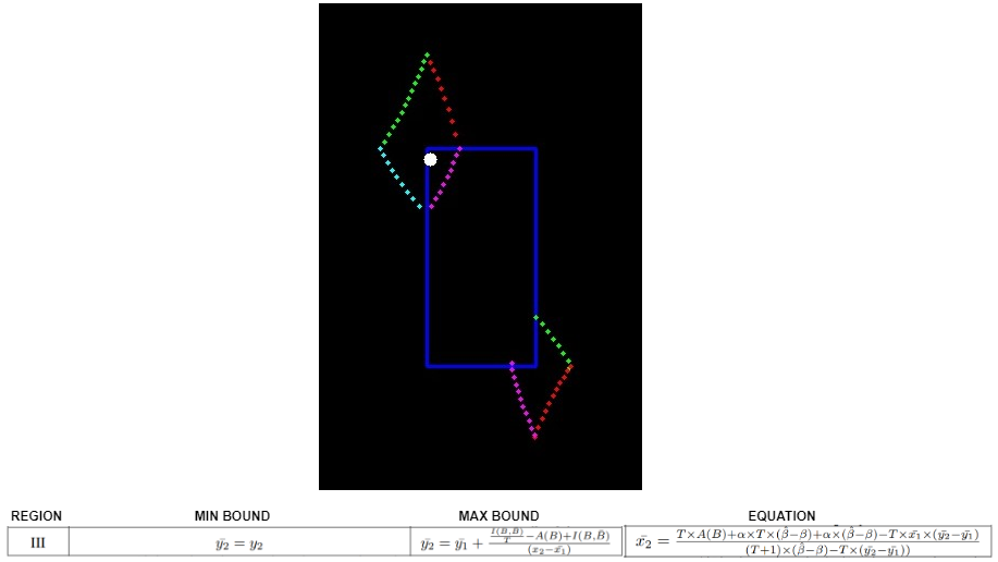 source) of Quadrant 3
源 )
#3rd Quadrant Boundary Points Generationy2BL = np.arange(limitBottomY, box[3] - IoULimitPrecision, step=-IoULimitPrecision)yBnew = np.minimum(y2BL, box[3])x2BL = IoU * boxArea + xA * IoU * (yBnew - yA) + xA * (yBnew - yA) - IoU * proposedx1 * (y2BL - proposedy1)x2BL /= ((IoU + 1) * (yBnew - yA) - IoU * (y2BL - proposedy1))
source) of Quadrant 3
源 )
#3rd Quadrant Boundary Points Generationy2BL = np.arange(limitBottomY, box[3] - IoULimitPrecision, step=-IoULimitPrecision)yBnew = np.minimum(y2BL, box[3])x2BL = IoU * boxArea + xA * IoU * (yBnew - yA) + xA * (yBnew - yA) - IoU * proposedx1 * (y2BL - proposedy1)x2BL /= ((IoU + 1) * (yBnew - yA) - IoU * (y2BL - proposedy1))
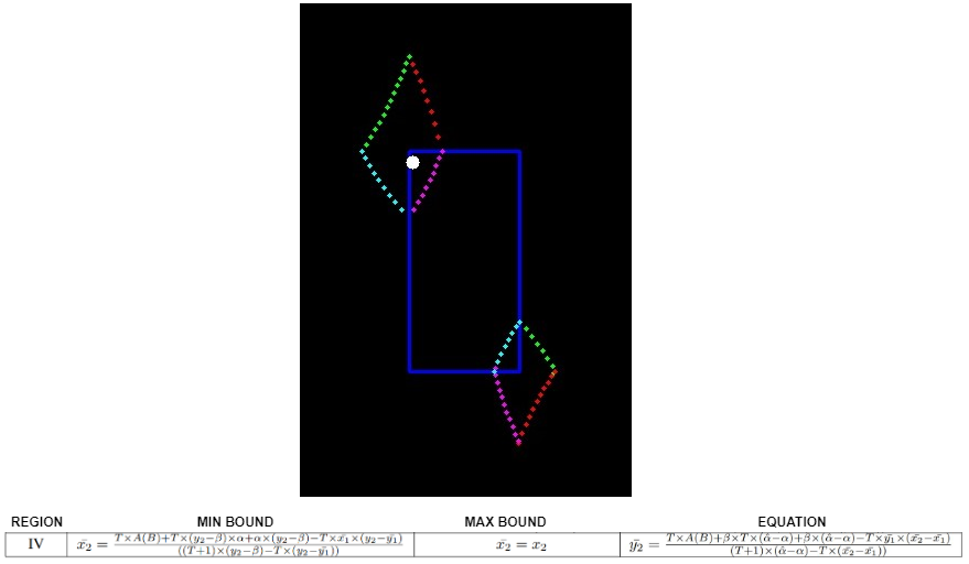 source) of Quadrant 4
源 )
#4th Quadrant Boundary Points Generationx2TL = np.arange(limitLeftX, box[2] + IoULimitPrecision, step=IoULimitPrecision)xBnew = np.minimum(x2TL, box[2])y2TL = IoU * boxArea + IoU * (xBnew - xA) * yA + yA * (xBnew - xA) - IoU * proposedy1 * (x2TL - proposedx1)y2TL /= ((IoU + 1) * (xBnew - xA) - IoU * (x2TL - proposedx1))
source) of Quadrant 4
源 )
#4th Quadrant Boundary Points Generationx2TL = np.arange(limitLeftX, box[2] + IoULimitPrecision, step=IoULimitPrecision)xBnew = np.minimum(x2TL, box[2])y2TL = IoU * boxArea + IoU * (xBnew - xA) * yA + yA * (xBnew - xA) - IoU * proposedy1 * (x2TL - proposedx1)y2TL /= ((IoU + 1) * (xBnew - xA) - IoU * (x2TL - proposedx1))
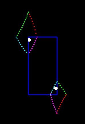 Fig-5(e): Output and Equation of Quadrant 1
图5(e):象限1的输出和方程
Fig-5(e): Output and Equation of Quadrant 1
图5(e):象限1的输出和方程
Since we have the bottom right boundary point feasible space (polygon2) can be defined. If the point lies in the feasible space it is a valid point (example point is shown in Fig-4). 由于我们具有右下边界点,因此可以定义可行的空间(polygon2)。 如果该点位于可行空间中,则它是有效点(示例点如图4所示)。 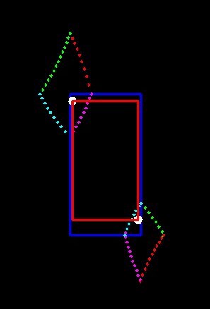 Fig-6 red box is synthetic bounding box and blue box is ground truth box
图6红色框是合成边界框,蓝色框是地面真实框
Fig-6 red box is synthetic bounding box and blue box is ground truth box
图6红色框是合成边界框,蓝色框是地面真实框
Finally, as we have both top-left sample point and bottom-right sample point we can generate bounding as shown in Fig-6 with 0.7 IoU threshold. 最后,因为我们同时具有左上采样点和右下采样点,所以可以生成如图6所示的具有0.7 IoU阈值的边界。 |
【本文地址】